Introduction
Accurate stack gas velocity measurement sits at the foundation of emissions compliance. Get it wrong, and every downstream calculation — mass emission rates for SO₂, NOₓ, CO₂ — inherits that error. The consequences range from invalid test results requiring costly retesting to permit violations if valid measurements aren't completed within required timeframes.
Power plants, refineries, cement kilns, pulp and paper mills — any stationary source with combustion gases exiting through a stack or duct faces this same measurement obligation. The regulatory burden is consistent across industries; the methods vary.
Two distinct compliance pathways exist: periodic manual source testing using Pitot tubes, and continuous monitoring systems (CEMS) that provide real-time flow data year-round.
This guide covers both. You'll find the regulatory framework, equipment requirements, step-by-step measurement procedure, key calculations, and where modern optical sensors fit into continuous monitoring for long-term compliance.
Key Takeaways
- Stack gas velocity determines how fast exhaust gases move through a stack, forming the basis for volumetric flow rate and mass emission calculations
- The standard manual method uses an S-type Pitot tube under EPA Method 2 (40 CFR Part 60, Appendix A-1); Ontario facilities follow Method ON-2
- Key inputs: velocity pressure (ΔP), absolute stack temperature, wet molecular weight, and absolute pressure
- Accuracy depends on site selection, equipment calibration, and detecting cyclonic or reverse flow
- Optical scintillation-based sensors provide continuous, no-maintenance monitoring for facilities with 24/7 CEMS requirements
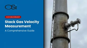
What Is Stack Gas Velocity Measurement?
Stack gas velocity measurement quantifies how fast exhaust or flue gases move through an industrial stack or duct, typically expressed in meters per second (m/s) or feet per second (ft/s). EPA Method 2 — formally titled "Determination of Stack Gas Velocity and Volumetric Flow Rate (Type S Pitot Tube)" — defines the standard approach. It supports both metric and English units, with the velocity constant Kp equal to 34.97 in metric and 85.49 in English units.
Where It Applies
The method covers any stationary source subject to air emissions regulations under 40 CFR Parts 60, 61, or 63. Common facility types include:
- Coal-fired and natural gas power plants
- Oil refineries and fluid catalytic cracking units
- Pulp and paper mills
- Cement kilns
- Chemical plants
- Aluminum smelters
Two Compliance Pathways
| Approach | Method | Frequency | Primary Purpose |
|---|---|---|---|
| Manual source testing | S-type Pitot tube, EPA Method 2 | Periodic (as required) | Compliance demonstrations, permit testing |
| Continuous monitoring | CEMS with permanent flow sensor | 24/7/365 | Ongoing reporting, Part 75 obligations |
Both pathways serve distinct compliance and operational purposes. Facilities with continuous emissions reporting obligations under Part 75 often need both running in parallel.
Why Stack Gas Velocity Measurement Matters
The Regulatory Framework
Two federal regulations govern most stack gas velocity measurement in the US:
- EPA Method 2 (40 CFR Part 60, Appendix A-1) — the reference method for manual velocity and volumetric flow testing at stationary sources
- EPA 40 CFR Part 75 — continuous monitoring, recordkeeping, and reporting requirements for SO₂, NOₓ, CO₂, volumetric flow, and opacity at affected electric generating units (EGUs) generally serving generators greater than 25 MW
The scale of Part 75 is significant. The Acid Rain Program initially covered 263 units at 110 plants, expanding to over 2,000 units in Phase II. According to EPA's 2023 Monitoring Insights analysis, stack-level monitoring covered 75% of NOₓ-reporting units, accounting for 78% of NOₓ emissions — a clear signal that stack-level flow data carries outsized compliance weight.

The Emissions Math Dependency
Total mass emission rate = gas velocity × stack cross-sectional area × pollutant concentration
An error in velocity cascades directly into every downstream figure. This is the calculation structure defined in Part 75 Appendix F, which converts concentration and volumetric flow into SO₂ and CO₂ mass emission rates.
If velocity is off by 10%, so is every mass emission result derived from it.
Operational Value Beyond Compliance
Velocity profiles reveal more than regulatory numbers. Plant engineers routinely use this data to:
- Identify combustion imbalances or fan degradation from uneven flow distributions
- Catch process upsets early through anomalous readings at known-stable sites
- Optimize combustion efficiency and reduce fuel waste
Each of these outcomes has a direct cost impact — measured in avoided downtime, reduced fuel consumption, or fines not incurred.
Equipment and Methods for Stack Gas Velocity Measurement
The S-Type Pitot Tube
The S-type (Stausscheibe) Pitot tube is the standard instrument for stack testing. Its larger openings resist plugging by particulate matter in dirty flue gas streams — unlike the standard Pitot tube, which clogs readily in real industrial exhausts despite performing well in clean gas.
EPA Method 2 construction and calibration requirements include:
- Material: Stainless steel construction
- External tubing diameter: 0.48 to 0.95 cm (3/16 to 3/8 in)
- Calibration coefficient (Cp): A baseline of 0.84 applies if the tube meets Method 2 dimensional specs; otherwise, calibration per Method 2 Section 10 is required
Differential Pressure Measurement
The manometer (inclined or electronic) measures the velocity pressure head (ΔP) between impact and static pressure ports. Key thresholds to observe:
- EPA Method 2: Requires a more sensitive gauge if average ΔP falls below 1.27 mm H₂O (0.05 in H₂O), or if sensitivity factor T exceeds 1.05 — data beyond these limits are unacceptable
- Ontario Method ON-2: ΔP fluctuations exceeding ±20% of the average at any traverse point render that point's data unacceptable
- Damping options: Capillary tubing or surge tanks may be used to reduce pressure fluctuations
Temperature Sensors
A calibrated thermocouple is fixed rigidly to the probe assembly, enabling simultaneous ΔP and temperature readings at each traverse point. EPA Method 2 requires:
- Calibration after each field use
- Agreement with a reference sensor within 1.5% of absolute temperature for field data to be considered valid
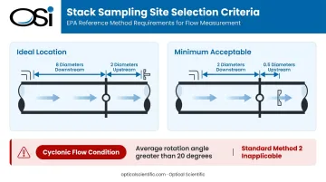
Site Selection
Sampling locations should meet Method 1 criteria:
- Ideal: At least 8 stack diameters downstream and 2 diameters upstream of any flow disturbance
- Minimum acceptable: At least 2 diameters downstream and 0.5 diameters upstream, with additional traverse points required
Cyclonic or swirling flow — defined as average rotation angles exceeding 20 degrees — renders standard Method 2 inapplicable. Alternatives include flow straightening vanes, stoichiometric flow calculation, or relocating to a suitable site. Confirming site suitability before deployment avoids costly remeasurement and keeps compliance data defensible.
How to Measure Stack Gas Velocity: Step-by-Step
The following procedure aligns with EPA Method 2 and standard Pitot traverse protocols. Each step builds on the last — skipping or rushing any phase risks data invalidation and failed compliance runs.
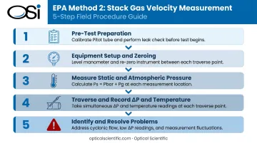
Step 1 — Pre-Test Preparation
Inspect and calibrate the Pitot tube as it will be used in the field, including the nozzle, thermocouple, and sheathing if part of the assembly.
Conduct a leak check: pressurize each Pitot tube opening until at least 7.6 cm H₂O (3.0 in H₂O) registers, then verify pressure holds within ±2.5 mm H₂O for at least 15 seconds. A post-test leak check is mandatory to validate the run.
Step 2 — Equipment Setup and Zeroing
Level and zero the manometer at the sampling location. Vibration and temperature changes cause drift — re-zero between traverse points. Record all readings on a standardized field sampling report from the start.
Step 3 — Measure Static and Atmospheric Pressure
Measure atmospheric (barometric) pressure with a calibrated barometer accurate to within 2.5 mm Hg (0.1 in Hg). Connect one manometer leg to the static tap to determine stack gas static pressure, then combine both values to calculate absolute stack pressure: Ps = Pbar + Pg, in consistent units.
Step 4 — Traverse and Record ΔP and Temperature
Move the probe to each defined traverse point. At each point, record ΔP and stack temperature simultaneously. Per Ontario ON-2, if ΔP fluctuates more than ±20% of the average at any point, that data is unacceptable — resolve the source of instability before continuing.
Step 5 — Identify and Resolve Common Problems
Three conditions require action before data collection can proceed:
- Cyclonic flow — Use alternate flow angle measurement procedures or relocate
- Very low ΔP — Switch to a more sensitive differential pressure instrument
- Persistent fluctuations — Stabilize the process or install dampening chambers; do not average through unstable readings
Key Calculations: From Stack Gas Velocity to Volumetric Flow Rate
Absolute Stack Gas Pressure
Ps = Pbar + Pg
Where Pbar is barometric pressure and Pg is stack static gauge pressure, both in consistent units (mm Hg or kPa). This combined absolute pressure feeds directly into the velocity equation.
Average Stack Gas Velocity
EPA Method 2 Equation 2-7:
Vs = Kp × Cp × (Σ√ΔPᵢ / n) × √(Ts / (Ps × Ms))
Where:
- Kp = unit constant (34.97 metric, 85.49 English)
- Cp = Pitot tube calibration coefficient
- ΔPᵢ = velocity pressure at each traverse point
- Ts = average absolute stack temperature (K or °R)
- Ps = absolute stack pressure
- Ms = wet-basis molecular weight (kg/kmol or lb/lb-mol)
Molecular weight requires companion gas composition analysis and cannot be assumed. Moisture content must also be determined from separate test methods before velocity can be accurately calculated.
Dry Standard Volumetric Flow Rate
EPA Method 2 Equation 2-8:
Qsd = 3600 × (1 - Bws) × Vs × A × (Tstd × Ps) / (Ts × Pstd)
Where Bws is the fraction of water vapor, A is the stack cross-sectional area, and Method 2 standard conditions are Tstd = 293 K and Pstd = 760 mm Hg. Dry standard reporting is the basis for permit compliance comparisons and long-term emissions load calculations across facilities.
Practical Velocity Benchmarks
EPA stack-sampling technical guidance identifies 1,000 to 5,000 ft/min as the normal working range for industrial stack gas velocity measurement. Velocities below 1,000 ft/min fall into low-range territory where standard Pitot tube sensitivity becomes a limiting factor.
Source-specific data points: a kraft process recovery boiler tested at approximately 2,746 ft/min; a wet-process cement kiln recorded approximately 5.28 ft/sec (~1,060 ft/min). These are facility-specific values, not category norms, but they give engineers a practical sanity check when evaluating traverses.
How OSI's Optical Flow Sensors Simplify Stack Gas Monitoring
Periodic Pitot tube testing answers compliance questions at a point in time. For facilities with continuous monitoring obligations under EPA 40 CFR Part 75, periodic testing alone doesn't close the gap. Repeated source testing contractor campaigns add up quickly — in cost, scheduling, and logistics.
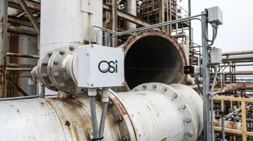
Optical Scientific (OSI) developed the OFS (Optical Flow Sensor) series in 2000 specifically to address this gap, targeting continuous stack gas flow monitoring at power plants for Part 75 compliance. Clients including the EPA, Duke Energy, Dominion Virginia Power, ExxonMobil, and Chevron have deployed OFS systems for exactly this purpose.
How the Technology Works
The OFS uses patented optical scintillation measurement: infrared light passes across the stack, and the sensor detects how thermal turbulence in the gas stream modulates that light. A DSP-based algorithm, certified by NIST and supported by over 20 million hours of observation data, converts those fluctuations into velocity. Because the measurement reads turbulence directly:
- No compensation needed for temperature, pressure, gas density, or moisture
- No differential pressure ports to plug or drift
- Accurate even at high particulate loads or variable opacity
OFS Series Models
| Model | Range | Best For |
|---|---|---|
| OFS-2000 | 0–100 m/s | Standard stack gas monitoring, Part 75 CEMS |
| OFS-2000F | 0.03–170 m/s | Flare stacks, thermal oxidizers, incinerators |
| OFS-2000W | 0–100 m/s | Wet scrubbers, bag houses, high opacity environments |
All models deliver ±2% accuracy, operate from -50°C to 60°C, and carry an MTBF exceeding 80,000 hours. The OFS-2000W adds Automatic Gain Control (AGC) to compensate for opacity variations from particulate matter or moisture. Since 1999, no OFS system has recorded a calibration fault.
Operational Advantages Over Periodic Testing
- Eliminates mechanical failure modes: no moving parts, no differential pressure ports to clog or drift
- Ships factory pre-calibrated with built-in automatic calibration checks; no field calibration required
- Requires only semi-annual window cleaning; internal diagnostics alert users when cleaning is actually needed
- Delivers 24/7 data via RS-232 and Modbus RTU standard, with optional RS-485, Ethernet, or cellular; one-minute updates with 10-second instantaneous readings
- Installs via standard ANSI 4-inch pipe flange with hot-tap capability: no process shutdown, no pressure drop
These operational characteristics translate directly into business value. At a terminal loading facility in southern California, OFS-2000 deployment enabled real-time NOx mass emission calculation, supporting a permit modification that eliminated unnecessary loading shutdowns. The system paid for itself through increased throughput alone.
Part 75 compliance depends on meeting performance specifications — including a RATA relative accuracy of 10% or less — not on technology type. Facilities considering OFS for CEMS applications should work through site-specific certification requirements with OSI's engineering team.
Frequently Asked Questions
How do you measure stack velocity?
Insert a calibrated S-type Pitot tube into the stack at defined traverse points, then measure the differential pressure (ΔP) between impact and static ports alongside stack temperature at each point. Apply the Method 2 velocity equation using ΔP, Pitot coefficient, absolute temperature, molecular weight, and absolute pressure to calculate velocity at each point, then average across the traverse.
How do you calculate stack flow rate?
Multiply the average stack gas velocity (averaged across all traverse points) by the stack cross-sectional area, then apply corrections for moisture content and reference pressure/temperature conditions. EPA Method 2 reports flow on a dry basis at standard conditions (293 K, 760 mm Hg) so results are comparable across sources and time periods.
What is the rule of thumb for gas velocity in industrial stacks?
EPA stack-sampling technical guidance places the normal working range at 1,000 to 5,000 ft/min. Below 1,000 ft/min, standard Pitot tube sensitivity may be insufficient and a more sensitive instrument is required. Readings outside this range are still usable, but verify that site conditions and equipment match the actual velocity before relying on them.
What is the difference between an S-type and a standard Pitot tube?
The standard Pitot tube is more accurate in clean gas streams but prone to plugging by particulate matter. The S-type has larger openings that resist plugging in dirty flue gas, making it the standard instrument for most industrial stack testing. The trade-off is that the S-type requires a separate calibration coefficient (Cp), whereas the standard Pitot tube uses a fixed coefficient of approximately 0.99.
What US regulations govern stack gas velocity measurement?
EPA Method 2 (40 CFR Part 60, Appendix A-1) is the primary federal reference method for manual stack gas velocity testing at stationary sources. EPA 40 CFR Part 75 governs continuous flow monitoring at electric generating units subject to the Acid Rain Program. Optional methods 2F, 2G, and 2H — covering 3-D probes, 2-D probes, and near-wall velocity decay — are also approved under Parts 60, 61, and 63.
What causes fluctuating velocity pressure readings during stack testing?
Per Ontario Method ON-2, ΔP fluctuations exceeding ±20% of the average at a traverse point indicate process or upstream equipment instability — not normal stack turbulence. Data collected under those conditions are unacceptable. The process must be stabilized, or dampening measures (capillary tubing, surge tanks) applied, before valid measurements can be collected.