ARC Advisory Group estimates that downtime costs the process industries roughly $1 trillion per year — and inaccurate flow measurement is a persistent contributor. Getting turbulent flow measurement right requires understanding the physics, selecting the right technology, and implementing it correctly.
This guide covers what turbulent flow actually is, how to predict it using the Reynolds number, which measurement technologies perform well (and which don't), and a practical step-by-step framework for getting accurate readings in demanding industrial environments.
Key Takeaways
- Turbulent flow is characterized by chaotic, irregular fluid motion with eddies and vortices — the dominant flow state in most industrial applications.
- The Reynolds number (Re = ρvL/μ) predicts flow regime: laminar below ~2,300, transitional between 2,300–4,000, and turbulent above ~4,000.
- Conventional meters (mechanical, differential pressure) struggle with turbulent, high-particulate, or high-temperature flows.
- Non-intrusive sensors with no moving parts offer the best long-term accuracy in harsh industrial environments.
- Proper site characterization, sensor selection, installation, and validation are all essential steps that directly affect measurement accuracy.
What Is Turbulent Flow?
The Physics Behind the Chaos
Turbulent flow is a fluid motion state defined by chaotic, irregular velocity and pressure changes. Rather than moving in smooth, parallel layers — as in laminar flow — turbulent fluid parcels follow unpredictable three-dimensional paths, forming eddies and vortices across a wide range of scales.
As NASA defines it, the Reynolds number characterizes which regime a flow occupies:
Re = ρVL/μ
Where ρ is fluid density, V is mean velocity, L is the characteristic length (typically pipe diameter), and μ is dynamic viscosity.
The standard engineering thresholds for pipe flow:
| Reynolds Number | Flow Regime |
|---|---|
| Re < 2,300 | Laminar |
| Re 2,300 – 4,000 | Transitional |
| Re > 4,000 | Turbulent |
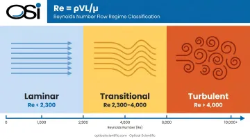
Most industrial pipe flows, ducts, and stacks operate at Reynolds numbers far above 4,000. ASME MFC-3M specifies minimum Re requirements for differential pressure meters ranging from 10,000 to 200,000 depending on device type. Those thresholds underscore just how routinely industrial flows operate deep within the turbulent regime.
Why Turbulence Complicates Measurement
Three physical features of turbulent flow create measurement difficulty:
- Velocity profiles are flat, not parabolic — unlike laminar flow, turbulent profiles shift significantly with upstream disturbances such as bends, valves, and expansions
- Point measurements are unreliable — velocity and pressure at any fixed location fluctuate randomly with time, as documented by NPTEL's fluid mechanics references
- Kolmogorov energy cascade transfers turbulent energy from large eddies down to small dissipative scales, generating noise from sub-hertz fluctuations up through kilohertz ranges
The practical result: a sensor that assumes a stable, uniform profile can introduce systematic flow measurement errors of 5–15% or more in highly turbulent conditions — enough to cause regulatory compliance failures in EPA-monitored stack applications.
How Turbulent Flow Is Measured: Key Methods and Technologies
Before selecting any measurement technology, engineers should calculate or estimate the Reynolds number using available fluid data. Skipping this step — and simply installing whatever meter is on hand — is one of the most common causes of persistent measurement error.
Differential Pressure (DP) Flow Meters
Orifice plates, Venturi tubes, and flow nozzles infer flow rate from the pressure drop across a restriction. They can function accurately in turbulent flow, but they come with strict prerequisites:
- ASME MFC-3M sets minimum Reynolds number thresholds: ≥10,000–20,000 for orifice plates and flow nozzles, ≥200,000 for Venturi tubes
- Upstream straight-pipe requirements are substantial — an orifice plate at beta ratio 0.75 requires 30D of straight pipe after a single 90° elbow for zero added uncertainty
- A peer-reviewed study of ultrasonic meters behind a 90° bend found systematic errors up to 10.8% at less than 8D — illustrating how severe profile distortion can be when straight-run requirements aren't met
DP meters are cost-effective and well-understood, but they demand careful installation and are not suitable for gas flows with high particulate loading that can clog pressure taps.
Mechanical and Turbine Meters
Turbine and propeller meters use a spinning rotor to infer velocity. The problems in turbulent flow are predictable:
- Velocity fluctuations cause rotor vibration and bearing wear over time
- High-particulate flows accelerate mechanical degradation
- Vortex shedding meters handle stable turbulent flow reasonably well, but Emerson notes that K-factor nonlinearity appears below Re ~20,000 for liquids and ~15,000 for gases — requiring careful range matching
For high-temperature or high-particulate turbulent gas flows, moving-part meters face accelerated degradation and frequent maintenance intervals.
Ultrasonic and Electromagnetic Flow Meters
Ultrasonic transit-time meters are non-intrusive and perform well in fully developed turbulent pipe flow. Key considerations:
- Clamp-on ultrasonic meters (Siemens, for example) report accuracies of 0.5%–1.0% under good installation conditions
- Fouling can add ≥0.5% uncertainty (per KROHNE), and pipe contamination alters both speed-of-sound readings and signal strength
- Electromagnetic meters work well with conductive liquids (water, acids, slurries) in turbulent conditions, but are not applicable to gas flow — including stack gas
Both technologies require adequate upstream straight runs. The 90° bend study cited above showed errors dropping from 10.8% at 0D to 0.7% at 12D. In retrofit applications where 12D–30D of straight pipe is physically unavailable, even a well-selected meter will produce unreliable readings.
Optical Scintillation Sensors
Optical scintillation flow measurement detects the fluctuating light signal produced by refractive index variations as turbulent fluid passes through an optical beam path. Unlike the technologies above, the method relies on turbulence itself to generate the signal — making it a natural fit for high-turbulence gas flow applications where other meters struggle.
A 2014 Journal of Environmental Protection study validated this principle for flue-gas velocity measurement, using two parallel optical paths and cross-correlation time delay; average velocity agreement was 7.62 m/s vs. 7.61 m/s against Pitot-tube reference.
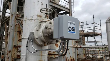
OSI's OFS series applies this principle using an all-digital signal processing architecture (DSP-based, with no temperature-sensitive analog components). Key specifications:
- OFS-2000: 0–100 m/sec range, ±2% accuracy
- OFS-2000F: 0.03–170 m/sec, designed for flare stack applications
The measurement is unaffected by temperature, pressure, gas density, moisture, or opacity. In the high-temperature, high-particulate conditions where turbine meters degrade and DP taps clog, the OFS series continues operating without scheduled maintenance.
A Practical Step-by-Step Approach to Turbulent Flow Measurement
Each step here shapes the next — skipping flow characterization and jumping straight to sensor selection is the most common cause of persistent measurement errors discovered months into operation.
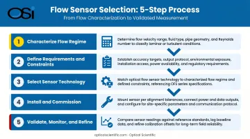
Step 1 – Characterize the Flow Regime
Calculate the Reynolds number using fluid density, dynamic viscosity, mean velocity, and pipe/duct diameter. Document the expected range — minimum, normal, and maximum flow conditions. Turbulence intensity varies with flow rate, and that variation determines which sensors stay accurate across all operating conditions.
Step 2 – Define Measurement Requirements and Constraints
Establish non-negotiables before evaluating any technology:
- Accuracy requirement — EPA 40 CFR Part 75 requires flow monitor calibration error ≤3.0% of span and RATA relative accuracy ≤10.0%
- Output type — volumetric vs. mass flow, data update rate, communications format
- Environmental constraints — temperature range, particulate loading, corrosive compounds, humidity
- Installation access — available straight-pipe run length, stack diameter, flange access
- Maintenance capacity — how often can the site realistically service the meter?
Step 3 – Select the Appropriate Sensor Technology
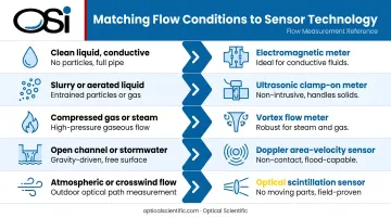
Map the constraints from Step 2 against technology capabilities:
| Condition | Recommended Technology |
|---|---|
| Clean liquid, conductive | Electromagnetic meter |
| Clean liquid or gas, good straight runs | Ultrasonic transit-time |
| General turbulent gas, adequate straight runs | DP meter (orifice/Venturi) |
| High-temperature, high-particulate stack gas | Optical scintillation (no moving parts) |
| Flare stack (wide velocity range) | Optical scintillation (extended range) |
Step 4 – Install and Commission Correctly
Improper installation causes the majority of field measurement errors — even when the correct meter type has been chosen. Critical factors:
- Meet the upstream/downstream straight-pipe run requirements for the specific meter and fitting geometry
- Follow manufacturer mounting angle and orientation specifications
- Commission against known reference conditions (EPA Method 2 Pitot traverse for stack applications)
- Verify communications integration with SCADA/DCS/CEMS data acquisition systems
Step 5 – Validate, Monitor, and Refine
After commissioning, confirm the readings make sense:
- Cross-reference against a secondary meter, Pitot traverse, or known process mass balance
- Establish data quality flags for readings outside expected turbulence intensity ranges
- Define a re-calibration schedule appropriate to the technology (optical scintillation instruments, for example, are drift-free by design)
- Review measurement performance after any process changes that could alter flow conditions. New upstream fittings, shifts in fluid composition, or changes in load demand all affect turbulence characteristics and may require recalibration.
Common Challenges in Turbulent Flow Measurement
Transitional flow uncertainty. When Re falls between ~2,000 and 4,000, flow can alternate between laminar and turbulent states unpredictably. In this range, meter accuracy suffers because the relationship between average velocity and centerline velocity shifts — a problem that hits insertion-type and thermal meters hardest. Two practical approaches address this:
- Design the system to operate clearly above or below the transitional range
- Select a sensor validated for performance in both laminar and turbulent states
Velocity profile distortion. Fully developed turbulent flow has a relatively flat velocity profile, but upstream disturbances (bends, valves, expansions) create swirl and asymmetry. Correction strategies include:
- Extended straight-pipe runs (following ASME MFC-3M or ISO 5167-2 table values for the specific meter and fitting geometry)
- Flow conditioners installed upstream
- Multi-path or cross-path averaging sensors that inherently average across the profile
Harsh environment degradation. High-temperature stack gases carry particulates and corrosive compounds that erode mechanical components, clog pressure ports, and coat optical surfaces. Strategies that work:
- No-moving-parts sensor architectures (primary defense against wear)
- Automatic Gain Control circuitry to compensate for optical surface contamination
- High-purge spools for especially challenging environments
- Built-in self-diagnostics that alert operators when maintenance thresholds are reached
How OSI Can Help with Turbulent Flow Measurement
OSI (Optical Scientific, Inc.) has specialized in optical scintillation-based flow measurement since 1985. The company's OFS series was developed specifically to address the measurement challenges that defeat conventional technologies in industrial turbulent flow environments — stack gas monitoring for EPA 40 CFR Part 75 compliance at power plants, flare stack measurement for refineries, and atmospheric turbulence monitoring for NASA, NOAA, and the U.S. military.
The OFS series addresses the core problems of harsh turbulent flow measurement directly:
- No moving parts — eliminates the wear and degradation that cause mechanical meters to fail in high-velocity, high-particulate gas flows
- ±2% accuracy across the full measurement range, maintained in high temperatures, variable opacity, and dust-laden conditions
- No calibration required — the optical scintillation measurement is drift-free by design; the system's NIST-certified algorithm has shown no calibration fault in any OFS deployment since 1999
- Minimal installation footprint — requires only 2 upstream and 1 downstream pipe diameters, significantly less than DP meters or ultrasonic clamp-on devices after a fitting
- Built-in continuous self-diagnostics — fault alarm triggers if drift exceeds 3% from normal parameters, providing data quality assurance for compliance applications
- MTBF exceeding 80,000 hours — field-proven through major utility customers including Duke Energy, Dominion Virginia Power, and Detroit Edison
Three OFS variants cover different turbulent flow applications:
| Model | Velocity Range | Key Application |
|---|---|---|
| OFS-2000 | 0–100 m/sec | General stack gas, thermal oxidizers, air ducts |
| OFS-2000F | 0.03–170 m/sec | Flare stacks (extreme velocity variation) |
| OFS-2000W | 0–100 m/sec + AGC | High-opacity: wet scrubbers, bag houses |
Each variant is designed for a specific set of real-world conditions. Contact OSI at info@opticalscientific.com or +1 301-963-3630 to discuss which OFS model fits your application.
Frequently Asked Questions
How do you measure turbulent flow?
Turbulent flow is measured using instruments suited to chaotic, high-velocity conditions — including differential pressure devices (with adequate straight-pipe runs), ultrasonic transit-time meters, vortex shedding meters, and optical scintillation sensors. Sensor selection depends on fluid type, temperature, particulate loading, and required accuracy.
What if Reynolds number is between 2,000 and 3,000?
A Reynolds number in this range falls in the transitional regime, where flow unpredictably shifts between laminar and turbulent states — and most meters struggle with the changing velocity profile. Design the system to operate clearly above or below this range, or select a sensor validated for transitional conditions.
What Reynolds number indicates turbulent flow?
Turbulent flow is generally established when Re exceeds approximately 4,000 in pipe flow. Values below 2,300 indicate laminar flow; the range between represents a transitional zone. Exact thresholds vary with geometry, surface roughness, and fluid properties — and many meter standards set higher minimum Re thresholds for accurate performance.
Why is turbulent flow harder to measure than laminar flow?
Turbulent flow's fluctuating velocity profile, pressure oscillations, and three-dimensional vortex structures make it far harder to characterize than laminar flow's smooth parabolic profile. Most sensors measure at a point or cross-sectional average, and turbulence creates real uncertainty about whether that reading represents true bulk flow.
What types of flow meters work best in turbulent conditions?
Differential pressure devices, ultrasonic transit-time meters, electromagnetic meters (for conductive liquids), and optical scintillation sensors all perform well in fully developed turbulent flow. In harsh environments with high temperatures or particulates, non-intrusive optical methods with no moving parts deliver the best long-term accuracy.